« Previous
Next »
 Select the Table data Header Row>> Click on Data Tab >> Click on Filter button (sort and filter group).
Use filter with simple Example:
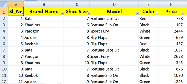
Suppose you are to seeing data where Shoe Size is 9. Then you can set filter to do this and follow the below steps.
« Previous
Next »
MICROSOFT EXCEL 2013
FILTERS IN MS EXCEL
Filter is a MS excel tools which allow you to quickly extract certain data from your spreadsheet. It actually hides the rows or columns containing data that do not meet the filter criteria you define. Excel has two features for filtering i.e. AutoFilter and Advance Filter.
AUTOFILTER
It is very easy to extract data from your spreadsheet.
Select the Table data Header Row>> Click on Data Tab >> Click on Filter button (sort and filter group).
Use filter with simple Example:
Suppose you are to seeing data where Shoe Size is 9. Then you can set filter to do this and follow the below steps.
- Place a cursor on the Header Row
- Choose Data Tab
- Click on Filter button to set Filter
- Click the drop-down arrow of shoe size column Header and remove the check mark from Select All which unselects everything.
- Then select the check mark for size 9 which will filter the data and displays data of shoe size 9. Some of the row numbers are missing (hidden) and the drop down arrow graphic will changed and marked as filtered icon.
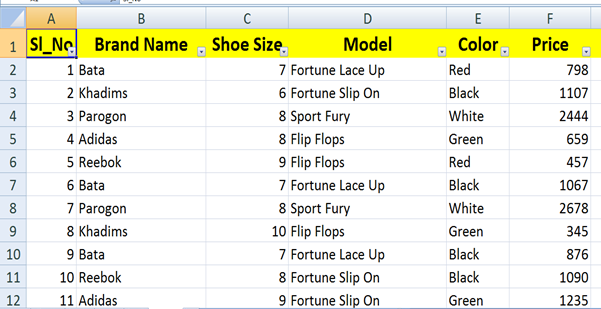
- Below is the data sheet and enter it in your excel sheet.
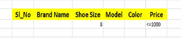
- Create the criteria range on different location of the same sheet as below according to this example.
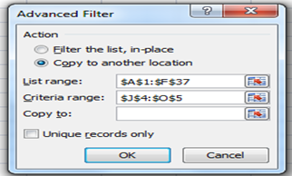
- Click any single cell inside data table >>Click on advance filter option from sort and filter group of Data menu ribbon. After you click the Advanced Filter dialog box will display as right.
- Click on the Criteria range box and select criteria range.
- Click on radio button to active Copy to another location as below.
- Click on copy to box and click on the place where you want to display your results in the same sheet.
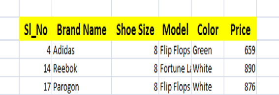
- Click on ok button and display the result you want then you final answer will display like below.
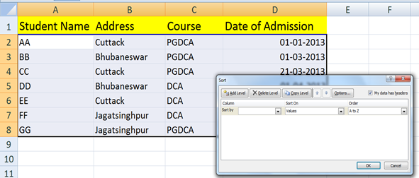
- Select the Column by which you want to sort data.
- Choose Data Tab.
- Click on Sort button to open Sort dialog box as illustrated below.
- Select the desired option in Sort dialog box to sorting data from database.
- Select the column you want to be sort.
- Select an option to sort based on a condition which are listed below:
- Values: Alphabetically or numerically
- Cell Color Based on Color of Cell
- Font Color Based on Font color
- Cell Icon Based on Cell Icon
- Select an Order like ascending or descending.
- Click on OK button to sort.
Multiple Filters
You can filter the records by multiple conditions i.e. by multiple column values. Suppose after size 9 is filtered you need to have filtered where color is equal to Black, then click on color drop down arrow and uncheck the select all and check the color black.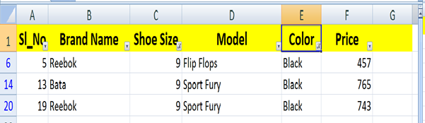
Advance Filter
This displays the result set of a query based on a complex criteria which you specify. Advance filter only display the record which meet the complex criteria.Ex: Suppose you display the different companies shoe which price <= 1000 and Shoe Size is 8. The advance filter helps you to searches particular shoes as your criteria and follows the below steps:
SORTING IN MS EXCEL
Sorting data in MS Excel rearranges the rows based on the contents of a particular column. You may want to sort a table to put names in alphabetical order. Or, maybe you want to sort data by Amount from smallest to largest or largest to smallest.To Sort the data follow steps.